Introduction to BSP Trees

Author: Антон В. Звягинцев
Source: https://gamedev.ru/code/articles/BSP/

---

Scope

This article gives a fairly detailed overview of the BSP (Binary Space Partitioning) algorithm and its main variations. Some of the material (particularly around node-based BSP in the render path)  is now outdated; newer hardware has changed the original algorithms, and today the BSP tree itself plays a smaller role in rendering than it once did. The fundamentals are still worth covering.

Prerequisites

To follow the material you need basic vector geometry — the dot product, the cross product, and the plane equation — plus familiarity with tree and linked-list data structures and how they are built. Code samples are C/C++-style pseudocode or C/C++ functions, and the full examples in Part Two use C++. You also need to be comfortable with recursion.

A note on the code

The examples are not optimized; readability was prioritized over performance. This is not a step-by-step tutorial — you will not find a complete BSP compiler implementation here — but rather a presentation of the core ideas and principles.

What BSP is

Binary Space Partitioning is a recursive, hierarchical subdivision of an n-dimensional space. The tree is built by using a hyperplane to split space into two parts. A hyperplane in n-dimensional space is an (n−1)-dimensional object that divides the space in two: in 3D it is a plane, in 2D it is a line.

The tree is built ahead of time by one or more utilities collectively called a BSP compiler.

Note: In Quake engines, the single utility qbsp builds the BSP tree from the input polygon set. Other utilities handle separate tasks, such as generating lightmaps.

Because the tree is precomputed, a key limitation is that it cannot be modified in real time during execution.

Programs that use BSP trees in some form include:

• Doom and games on its engine (Doom II, Heretic, Hexen)
• Unreal and games on its engine
• Quake 1, 2, and 3, and games built on their engines
• Hexen 2, Half-Life 1–2 (Quake 1 engine lineage)
• Sin, Kingpin (Quake 2 engine)
• Jedi Knight II: Jedi Outcast, Medal of Honor, Star Trek titles (Quake 3 engine)
• Shogo: Mobile Armor Division, Blood 2, Aliens vs. Predator 1–2, Die Hard: Nakatomi Plaza, NOLF2 (LithTech 1–2)
• Doom 3
• ...and many others

A brief history

The name John Carmack is often treated as synonymous with BSP, but the algorithm predates his work.

Note: Carmack was likely the first to voice and implement PVS-data compression, including the use of bit vectors to represent it. PVS is discussed later.

The foundations of BSP were laid in 1969. In 1980–83, Fuchs et al. revisited those ideas and formalized what is now known as the Binary Space Partitioning tree. In 1991, Teller and Séquin proposed generating a PVS (Potentially Visible Set) to speed up visibility determination in a 2D orthographic setting, and in 1992 Teller described PVS generation for a polygonal 3D environment. In 1991, Chen and Gordon described an efficient front-to-back method of rendering a BSP tree, in contrast to the back-to-front approach used at the time.

Editor's note (accuracy): The original spelled Fuchs as "Funch" and dated the Teller–Séquin PVS work to 1990; it was published in 1991 ("Visibility Preprocessing for Interactive Walkthroughs," SIGGRAPH). The Chen–Gordon reference is correct ("Front-to-Back Display of BSP Trees," IEEE CG&A, 1991).

Chronology of the id Software engines relevant to Part Two:

• December 10, 1993 — Doom.
• October, 1994 — Doom II. Same engine and "2.5D" approach; effectively an expansion of the base version.
• June, 1996 — Quake. First title with true 3D and polygonal monsters. Open architecture with the built-in QuakeC language enabled mods and total conversions: platformers, racers, chess, football, an arcade flight simulator, and rule variants such as CTF, Team Fortress, and Head Hunters.
• December 1997 — Quake II. Split the fanbase (Q1 vs. Q2) and showed a large gap between the hardware-accelerated and software versions. Internally, its architecture differed only minimally from Quake 1. QuakeC was dropped; mods were now written in C and compiled to an OS dynamic library.
• December 2, 1999 — Quake III Arena. Hardware acceleration only. Heavy use of Bézier patches (a subset of NURBS). Returned to a virtual machine (QVM/QASM), while apparently still supporting OS dynamic libraries in early test builds.

ID1 titles before Doom did not use BSP. Wolfenstein 3D used ray casting (not to be confused with ray tracing).

Node BSP Tree

A node-based BSP tree addresses several problems that were more pressing historically but remain foundational:

• Drawing polygons (including overlapping ones) in the correct order — for example, far to near — which automatically handles transparent and semi-transparent polygons, since these must be drawn after whatever they overlap.
• No Z-buffer is required (applies specifically to the classic node-based BSP).
• With a small change to the data representation, you get near-free collision detection.

Building a tree by example

Because 2D and 3D BSP construction are identical in principle, the examples use a 2D case while keeping 3D terminology.

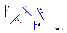
Figure 1 shows a top-down view of a typical game level. The red dot is the player/camera position (its orientation does not matter here). Blue lines are walls, with their normals shown. In this 2D world, wall height is ignored.

BSP construction rests on splitting space by the plane on which a given polygon lies. For simplicity, assume each wall is a single polygon. Take polygon b as the first splitter. In front of b's plane lie polygons d and e; polygon a lies behind it; polygon c is cut by the splitter.

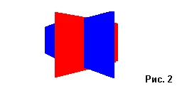
Note: Splitting by the splitter's plane solves a problem that simple depth-sort methods — such as the painter's algorithm — cannot. The painter's algorithm sorts polygons by distance, but the overlapping case shown in Figure 2 cannot be resolved correctly by it.

Consider Figure 3:

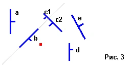
The first split cuts polygon c into c1 and c2; both inherit the parent's facing direction. After the first split we have two lists:

• In front of the splitter's plane: c2, d, e
• Behind the splitter's plane: a, c1

Polygon b is removed from the candidate list and placed in a tree node. We now recurse on each of the two lists until no polygons remain as input.

Take the front list — c2, d, e — and choose c2 as the splitter (the splitter is always chosen from within the list being processed).

Note: The choice of splitter is not arbitrary; the example uses an empirical pick. Choosing a good splitter is discussed later.

After this second split:

• In front of the splitter: d
• Behind the splitter: e

The third split processes the list a, c1 (the "behind" list from the first split), with a as the splitter:

• In front of the splitter: c1
• Behind the splitter: none

Continuing recursively produces the tree in Figure 4. That is the BSP tree.

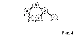
In the figure, children to the right of a node are in front of the parent splitter; children to the left are behind it. The root node holds polygon b. This is exactly the work a BSP compiler does: building the tree, resolving conflicts with overlapping and coplanar polygons, and choosing the splitter plane.

Note: It is common for several polygons to lie on the same plane. If one of them is used as the splitter, the coplanar polygons are simply stored together with the splitter in the same node. The case of coplanar polygons with opposite normals is handled later, in the sections on rendering and data-structure design.

Choosing a good splitter; balanced trees

Splitter selection involves a trade-off. To help rendering, you want to minimize how many polygons the splitter cuts, since each cut adds polygons to the scene. Many sources treat minimizing polygon and node counts as the primary goal. At the same time, you often want a balanced tree — one with roughly equal node counts on each side of the root (and, recursively, of every node, since each node is the root of its own subtree).

Why does imbalance matter? With an unbalanced tree, frame rate can swing sharply across different parts of the level. A classic BSP tree used only for rendering, with no algorithmic modifications, is not affected by this, because the entire tree is traversed and every polygon is drawn regardless of structure. The situation changes when the algorithm is extended — for example, using a Solid BSP variant for collision detection (covered later). Because a collision test descends to different depths in different parts of the level, one area might run at 60+ FPS and another below 10. A balanced tree keeps the frame rate roughly constant (say, around 30 FPS).

The theoretically best result comes from building every possible BSP tree for the input and picking the one with the fewest nodes — but this is computationally infeasible for real-world level sizes. The common practical approach is to iterate over all candidate splitter polygons and score each. This scoring does not account for how later splits will play out, so it cannot guarantee that the locally optimal splitter is globally optimal.

One scoring formula:

Score = abs(front - back)

where front and back are the polygon counts on each side of the splitter. The splitter with the lowest score wins. This targets balance at the current depth.

This ignores that a splitter may cut the polygons it crosses. To discourage cuts (and the polygon growth they cause), refine the formula:

Score = abs(front - back) + (splits * 8)

Here splits is the number of cuts, and 8 is a weighting coefficient. Lowest score still wins.

To also account for coplanar polygons — whether treating them as desirable or not is an open question, hence the ± sign:

Score = abs(front - back) + (splits * 8) ± coplanar

where coplanar is the number of polygons coplanar with the candidate splitter. Using minus gives splitters with more coplanar polygons a better chance of "winning."

Generalized:

Score = w1 * abs(front - back) + splits * w2 + coplanar * w3

where w1, w2, w3 weight each factor and may be negative (e.g., w3 = -1).

Rendering

Everything above holds for the 3D case as well. Returning to the example in Figure 1 and the tree in Figure 4, the traversal is best shown as pseudocode:

void RenderBSP(Node *node)
{
  int result = ClassifyPoint(camera_position, node->splitter_polygon);
  if (result == FRONT)
  {
    if (node->back != NULL)  RenderBSP(node->back);
    DrawPolygon(node->splitter_polygon);
    if (node->front != NULL) RenderBSP(node->front);
  }
  else
  {
    if (node->front != NULL) RenderBSP(node->front);
    DrawPolygon(node->splitter_polygon);
    if (node->back != NULL)  RenderBSP(node->back);
  }
  return;
}

ClassifyPoint() determines whether the camera is in front of or behind the current node's splitter plane (which we can always compute from the polygon stored in the node). DrawPolygon() draws the polygon. Until the algorithm is enhanced, the camera's orientation and view frustum are irrelevant — the whole tree is traversed. The first call receives the root node b.

Traversal for the camera position in Figure 1:

• Camera is in front of b → FRONT. Recurse into the back subtree first, which is node a.
• Camera is in front of a. Node a has no polygons behind it, so draw a.
• Node a has a front child → recurse into c1.
• c1 has no children → draw c1.
• Return through the recursion back to the first call.

The left side of the tree is now complete. Move to the right side:

• Back in the first call → draw b. Then recurse into c2.
• Camera is in front of c2 → recurse into e.
• e has no children → draw e.
• Return → draw c2.
• Recurse into d.
• d has no children → draw d.

Resulting draw order:

a, c1, b, e, c2, d

This is the back-to-front method: along any direction, the most distant polygons are drawn first. You can verify correctness by re-running the traversal with the camera elsewhere.

Back-to-front is not the only option. In Quake I's software renderer, Michael Abrash and John Carmack used a front-to-back approach: polygon edges were collected into a separate list and only their visible spans were rasterized. Its main advantage is no overdraw, but it suits software rendering more naturally than hardware rendering via OpenGL or Direct3D. Front-to-back also enables an early-out — ending traversal once every screen pixel has been rasterized — which is valuable on complex scenes.

Note: Quake I, II, and III use a leaf-based BSP tree with PVS for locating the player and for rendering. Leaf-based BSP is covered later.

Node culling

Imagine a large level to render. A BSP tree by itself does not simplify geometry or cull invisible faces, so with enough polygons the frame rate approaches zero. One remedy is the PVS algorithm (later). A simpler technique, computed at tree-build time, is bounding-volume culling.

Compute a bounding volume (box or sphere) for each node that also encloses all its descendants. Spheres are cheaper to compute and test but less precise. Then test each node against the view frustum at the start of RenderBSP():

void RenderBSP(Node *node)
{
  if (!IsInFrustum(node)) return;
  int result = ClassifyPoint(camera_position, node->splitter_polygon);
  // ...

and add the bounding-volume fields to the node structure.

Data structures

A minimal BSP node:

struct Node
{
  Polygon *splitter_polygon;
  Node    *front;
  Node    *back;
};

This pointer-based form has drawbacks — chiefly, it is awkward to serialize to disk without rebuilding. It is also better to precompute planes into a separate array so a plane can be shared among several polygons and speed up rendering. An index-based form:

struct Node
{
  int polyindex;
  int plane;
  int front;
  int back;
};

Here each member indexes into the corresponding array (polygons, planes, nodes). The examples below use the pointer form for clarity.

Handling coplanar polygons

Polygons lying on the splitter plane cannot be unambiguously classified and are stored in the same node as the splitter. To support the common case, extend the Polygon structure with two linked-list pointers:

struct Polygon
{
  ...
  Polygon *same;      // next coplanar polygon facing the same way
  Polygon *opposite;  // next coplanar polygon facing the opposite way
};

These form linked lists built during BSP compilation: same chains polygons facing the same direction as the splitter, opposite chains those facing the reverse. The rendering code becomes:

void RenderBSP(Node *node)
{
  Polygon *shared;
  int result = ClassifyPoint(camera_position, node->splitter_polygon);
  if (result == FRONT)
  {
    shared = node->splitter_polygon->same;
    if (node->back != NULL) RenderBSP(node->back);
    DrawPolygon(node->splitter_polygon);
    while (shared != NULL) { DrawPolygon(shared); shared = shared->same; }
    if (node->front != NULL) RenderBSP(node->front);
  }
  else
  {
    shared = node->splitter_polygon->opposite;
    if (node->front != NULL) RenderBSP(node->front);
    DrawPolygon(node->splitter_polygon);
    while (shared != NULL) { DrawPolygon(shared); shared = shared->opposite; }
    if (node->back != NULL) RenderBSP(node->back);
  }
  return;
}

Note: Part Two covers optimal in-memory and on-disk BSP layouts in more depth when building the Quake 1/2/3 renderers.

Solid Node BSP Tree

A Solid node BSP tree can be used efficiently for collision detection. Two differences from the plain node BSP:

• Where a plain tree stores NULL in front/back when a node has no children, the solid tree adds an extra child node (with front and back set to NULL) carrying an IsSolid flag. IsSolid marks space that the camera cannot or should not occupy.
• Polygons coplanar with the splitter are no longer stored in the splitter's node; they are instead added to the list of polygons in front of the splitter plane.

Consider the room in Figure 5 (a room example often used by Gary Simmons):

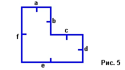
Build a Solid node BSP with b as the splitter. Polygon e is cut into e1 (left) and e2 (right), giving:

• In front of the splitter: a, f, e1
• Behind the splitter: c, d, e2

Take the front list and split again with a as splitter:

• In front of the splitter: f, e1
• Behind the splitter: none

There are no polygons behind a's plane, which signals inaccessible ("solid") space. So the back pointer is set to a new node with IsSolid = true and null children. Splitting again with f as splitter, only e1 lies in front, so the space behind f is also solid. The last remaining candidate, e1, must create two extra nodes, since neither side has further polygons. To keep the tree correct, only the back extra node gets IsSolid = true: when every polygon faces in front of the others (as with the list a, f, e1), the polygons form a convex volume, and the space inside that volume must not be marked solid.

The result is the tree in Figure 6:

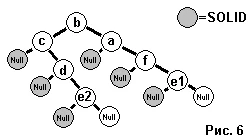
Gray circles mark the extra nodes with IsSolid = true.

Collision detection, briefly

Without any accelerating structure, collision must be tested against every polygon in the world. With a BSP tree, you descend from the root to the leaf node containing the object under test — just as in rendering — automatically discarding polygons along the way. Once you reach the relevant polygon, a simple ray trace tests intersection of a line with the polygon. The polygon is obtained from the parent node, since the extra (solid) nodes carry no polygon data. The line can be defined by two points — the object's current position and its intended destination.

Note: Gary Simmons uses a single tree for both rendering and collision (this is the Solid node BSP). That saves memory and can improve performance, but per-polygon collision precision is not always needed. Building a simpler, separate collision model — and a second, simpler BSP tree over it — is often a better choice.

BSP compiler math

The core functions a BSP compiler needs.

First, a function classifying a point relative to a plane. A plane is given by Ax + By + Cz + D = 0, where (A, B, C) is the plane normal.

Editor's note (accuracy): The original described D as "the distance to the origin." More precisely, D = -(N · P0) for a point P0 on the plane; the signed distance from the origin to the plane equals -D / |N|, and it equals |D| only when the normal is a unit vector. Treat D as a plane coefficient, not literally the distance, unless the normal is normalized.

Precompute planes for all polygons rather than computing them during rendering or compilation. The plane's normal equals the polygon's normal. For a triangle given by three vertices (counter-clockwise), compute two edges, take their cross product, and normalize:

void cp(float *v, float *v1, float *v2)
{
  v[0] = v1[1]*v2[2] - v2[1]*v1[2];
  v[1] = v1[2]*v2[0] - v2[2]*v1[0];
  v[2] = v1[0]*v2[1] - v2[0]*v1[1];
  return;
}

void norm(float *v)
{
  float c = 1 / sqrt(v[0]*v[0] + v[1]*v[1] + v[2]*v[2]);
  v[0] *= c;
  v[1] *= c;
  v[2] *= c;
  return;
}

Move D to the right-hand side:

Ax + By + Cz = -D

The left side is a dot product. So the point-classification function:

#define EPSILON  0.0001
#define ONPLANE  0
#define FRONT    1
#define BACK     2

int ClassifyPoint(float *p, float *v1, float *v2, float *v3)
{
  float result;
  float n[3], dir[3];
  for (int j = 0; j < 3; j++)
  {
    dir[j] = v1[j] - p[j];
  }
  getNormal(n, v1, v2, v3);
  result = dp(dir, n);
  if (result < -EPSILON) return FRONT;
  if (result > EPSILON)  return BACK;
  return ONPLANE;
}

dp() is the dot product. Because single-precision floating-point comparisons accumulate error, compare against an EPSILON constant rather than 0.0.

BSP compiler pseudocode

From the BSP FAQ:

void Build_BSP_Tree(BSP_tree *tree, list polygons)
{
  polygon *root = polygons.Get_From_List();
  tree->partition = root->Get_Plane();
  tree->polygons.Add_To_List(root);
  list     front_list, back_list;
  polygon *poly;
  while ((poly = polygons.Get_From_List()) != 0)
  {
    int result = tree->partition.Classify_Polygon(poly);
    switch (result)
    {
    case COINCIDENT:
      tree->polygons.Add_To_List(poly);
      break;

    case IN_BACK_OF:
      back_list.Add_To_List(poly);
      break;

    case IN_FRONT_OF:
      front_list.Add_To_List(poly);
      break;

    case SPANNING:
      polygon *front_piece, *back_piece;
      Split_Polygon(poly, tree->partition, front_piece, back_piece);
      back_list.Add_To_List(back_piece);
      front_list.Add_To_List(front_piece);
      break;
    }
  }

  if (!front_list.Is_Empty_List())
  {
    tree->front = new BSP_tree;
    Build_BSP_Tree(tree->front, front_list);
  }

  if (!back_list.Is_Empty_List())
  {
    tree->back = new BSP_tree;
    Build_BSP_Tree(tree->back, back_list);
  }
}

Notes on the functions:

• Get_From_List() returns the next input polygon. Here the root splitter is not tested for optimality — it is simply the first polygon in the list.
• tree->polygons.Add_To_List(root) stores the chosen polygon in the node; it is reused to store polygons found coplanar with the splitter.
• Classify_Polygon() reports whether a polygon is in front of (IN_FRONT_OF), behind (IN_BACK_OF), on (COINCIDENT), or split by (SPANNING) the splitter plane. Implement it by classifying each of the polygon's points with ClassifyPoint() and counting how many fall in front of, behind, and on the plane. If all points are in front (or on), the result is IN_FRONT_OF; all behind (or on) → IN_BACK_OF; all on → COINCIDENT; points on both sides → SPANNING. In the spanning case, Split_Polygon() cuts the polygon (implementation left as an exercise).

If either list is non-empty after classification, recurse into it.

Leaf BSP Tree

The most common BSP variant today is the leaf BSP tree, which differs substantially from node BSP in both structure and algorithm. Leaf BSP (with enhancements) is what Quake 1–3 use.

Key differences between node and leaf BSP:

• Nodes no longer carry level geometry. All geometry lives in the leaves — hence the name.
• When choosing a splitter, only its plane is stored in the node; the splitter polygon itself stays in the list of polygons in front of its plane and is flagged as "already used" so its plane cannot be reused for splitting.
• If an already-used splitter polygon is later cut by another splitter plane, both resulting pieces inherit the "used" status and cannot become splitters.
• After each split, if every polygon in an input list faces in front of the others, they form a convex, non-intersecting volume. That list becomes a leaf, and it is no longer used as input.

Applying this to Figure 5 gives:

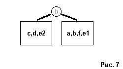
Using b's plane as the first splitter, polygon b is placed in the "front" list (not in the node — only the splitter plane goes into the node). After the first split, every polygon in each list already faces in front of the others, forming convex volumes and therefore leaves. Compare this with the Solid node BSP in Figure 6; a classic node BSP would not differ much from the solid variant.

Without enhancements, rendering a leaf BSP is the same as rendering a node BSP, but traversal is faster because a leaf BSP has far fewer nodes. No Z-buffer is needed: since a leaf's polygons do not intersect and each faces in front of the others, enabling back-face culling (OpenGL or Direct3D) yields a correct result regardless of draw order within a leaf.

A leaf BSP is much shallower and thus faster to traverse, but it does not solve one hard problem: render time still grows with level size, because traversing and drawing every polygon costs more as polygon count rises. In the solid node variant we used node culling to partly break this dependence; here we take a different route via the enhancements below.

PVS

PVS — Potentially Visible Set — is, roughly, an array holding, for each leaf, whether every other leaf is potentially visible from it.

Example: rooms A and B are joined by a bending corridor C such that A cannot see B and vice versa, but each room can see the corridor. Let A, B, C be leaves stored at indices 0, 1, 2. From A you can potentially see A and C; from B, only B and C; from C, all three. The PVS array:

       A B C
A PVS: 1 0 1
B PVS: 0 1 1
C PVS: 1 1 1

Note: PVS does not consider camera orientation and does not cull parts of the world outside the view frustum.

These are just boolean flags. With one byte per flag, the example needs 9 bytes. But with 10,000 leaves, 10,000 × 10,000 = 100,000,000 bytes ≈ 100 MB — unworkable. Remedies:

• PVS rows are often identical across leaves, so store unique rows only. The deduplicated array is called the cluster array, and each leaf holds an index into it.
• Use one bit per flag instead of a byte, cutting size 8×.
• Compress further if needed.

Zero Run-Length Encoding

Zero RLE is a variant of the long-established RLE family (PCX files, for instance, use RLE). It is simple enough to run in real time without a performance hit. Example encoded stream:

12, 0, 23, 2, 243, 0, 15

These 7 bytes encode 41 bytes of PVS information (and each byte covers 8 leaves). This is not an especially powerful compressor — it merely exploits the fact that PVS streams contain many zeros, since from any given leaf only a small fraction of leaves are typically visible.

Decompression: if a value is non-zero, write it unchanged. If a value is zero, the next byte gives the count of zero bytes to emit. So the stream above decodes to:

12, [23 zeros], 2, 243, [15 zeros]

(1 + 23 + 1 + 1 + 15 = 41 bytes.) The compression side is the inverse.

Rendering leaf BSP + PVS

Descend from the root to the leaf containing the camera. Then iterate over that leaf's PVS and render every leaf marked visible:

void RenderTree(int thisLeaf)
{
  for (int i = 0; i < NumberOfLeafs; i++)
  {
    if (Leafs[thisLeaf].pvsdata[i] == true)
    {
      RenderLeaf(i);
    }
  }
}

Note: A leaf is visible from itself, so when thisLeaf == i the condition should always be true.

With this approach a Z-buffer is required. Note that the root-to-leaf descent happens only once per frame — to find the leaf you are in — rather than traversing the whole tree.

Frustum culling

At compile time, store a bounding volume (box or sphere) in each leaf. Then, during rendering, after checking the PVS, discard leaves whose bounding volume falls outside the view frustum. (Detailed frustum-culling implementation is beyond this article's scope and is well documented elsewhere.)

Note: Whether frustum culling is worthwhile depends on the project. If the world is small and even modest GPUs can brute-force a Quake II–scale level at an acceptable frame rate, the CPU spent on culling tests might be better used elsewhere (e.g., AI). As the developer, weigh each algorithm against your target task and minimum hardware.

Portals

Portals — and dividing the world into zones or sectors (an area in Quake terminology) — are another way to make a BSP tree more efficient. Portals are independent of the BSP tree itself, but here we consider their use in a PVS BSP renderer.

Picture two rooms joined by a door rather than a corridor. When the door is open, each room can see the other; when closed, it cannot. A portal represents the door: if the portal is "closed," we skip the leaves in the other zone regardless of the PVS.

A portal need not be a literal door — it can be an invisible polygon at the boundary between two zones. In that case, portals pair well with frustum culling. Portals are a broad topic beyond this article's scope.

PVS and objects in the world

PVS is useful beyond determining visible geometry. It can limit which objects are simulated, or which data is transmitted, in a client/server networked game. Given the client's position, the server can readily determine whether an object — another player, an NPC, or an item — is potentially visible, since each such entity also resides in some leaf. Large amounts of data can therefore be filtered out before transmission.

Note: Quake II also used PHS — Potentially Hearable Set — a structure analogous to PVS, used by monster AI to determine from which parts of the level events could be heard.

Debugging tips

Following Dan Royer's advice, debug the renderer — and especially the BSP compiler — with the simplest possible models. Test these configurations:

• Two coplanar polygons.
• Two parallel polygons facing each other.
• Two parallel polygons, one behind the other.
• Two intersecting polygons.
• Two polygons sharing an edge but not coplanar.

Solid Leaf BSP Tree

To close the theory section, here is the solid variant applied to a leaf BSP, again using Figure 5:

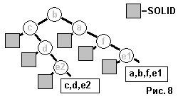
Compare Figure 8 with Figure 7. The main difference from a classic leaf BSP is that construction uses the planes of all polygons. Even though polygons a, b, f, and e1 form a convex volume, we keep using the planes of polygons that have not yet served as splitters. As a result there are never any back-leaves: every leaf behind a polygon's split plane represents inaccessible space, as in the Solid node BSP.

Closing

Do not use BSP algorithms for open spaces or for projects requiring wholesale destruction of the environment; the algorithm's nature makes those a poor fit. BSP trees are a powerful, flexible algorithm and data structure, but like any algorithm they have a proper domain of application.

For further reading, the paper An Investigation into Real-Time 3D Polygon Rendering Using BSP Tree is recommended.

---

Tags: mapping, level design